---
title: Welcome Back to LLM-Agents!
author: Jonathan Trnka
date: 2026-03-13
format:
html:
output-file: index.html
html-math-method: katex
code-fold: true
code-tools: true
code-fold-default: true
toc: true
toc-depth: 5
pdf:
code-block-bg: "red"
code-block-border-left: "blue"
code-fold: true
colorlinks: true
linkcolor: blue
number-sections: true
geometry: margin=1in
fontsize: 11pt
execute:
kernel: python3
cache: false
freeze: false
warning: false
message: false
error: false
echo: true
cite-method: citeproc
link-citations: true
suppress-bibliography: false
bibliography: LLM-Agentsref.bib
csl: apa.csl
---
# Recap
As you might recall from my previous presentation, I did a comparison between a baseline LLM (no agent capabilities) vs a single LLM-Agent (with all agent capabilities). The LLM Agent had capabilities such as API integration,
error check and self recovery, communication with other agents, and more.
Before I continue on, I would just like to go over this quote:
@agentsindex2026multiagent states,
"What is the difference between single agent and multi-agent AI systems?
The key difference is specialization and parallelism. A single AI agent handles all tasks sequentially within one context window; a multi-agent system distributes tasks across specialized agents working in parallel.
Multi-agent systems outperform single agents on complex, multi-domain workflows but underperform on simple sequential tasks where coordination overhead exceeds the efficiency gain."
# My objectives:
- Briefly explain the 3 "agents" I'll be using.
- Conduct and interpet 3 hypothesis tests.
- Interactive plots
- Provide further examples in specific areas of how to use LLM-Agents.
- Conclusion.
# Key Variables:
- <code>Baseline</code> = OPENAI gpt-4.1 model.
- <code>Single Agent</code> = Uses all 3 tools, has self recovery, replanning, prompts, API intergration all in a single agent.
- <code>Multi Agent</code> = Built simiarliy as the single agent but the process is broken up into multiple agents. One for planning/reasoning, one for execution/solving, one for final reviewing.
# Data and Research Question:
## Research Question:
**Based on speed, accuracy, and token usage, which performs better, a single agent or multi agent?**
## What dataset was used?
- I used a dataset of Bing queries from anonymous user. There were over 1 million queries gathered but I only downloaded about 5k and ended up using less than 100 for this presentation.
```{python}
import os
import sys
import pandas as pd
import ast
import io

from regression_metrics import run_all_regressions

# ---------------------------------------------------------
# Benchmark pipeline
#
# A re-run calls the OpenAI API once per query for each of the three
# systems and overwrites every result CSV, so it is opt-in. By default
# this report is built from the committed results of the original run.
# ---------------------------------------------------------
RUN_BENCHMARK = os.getenv("RUN_BENCHMARK", "").strip().lower() in {"1", "true", "yes"}

RESULT_FILES = [
    "single_agent_raw.csv",
    "multi_agent_raw.csv",
    "baseline_raw.csv",
    "correctness_scores.csv",
]

if RUN_BENCHMARK:
    # Imported here because it pulls in config.py, which requires API keys.
    from benchmark_wrapper import main
    _stdout = sys.stdout
    sys.stdout = io.StringIO()
    main(sample_size=100)
    sys.stdout = _stdout
    print("Benchmark re-run complete.")
else:
    _missing = [f for f in RESULT_FILES if not os.path.exists(f)]
    if _missing:
        raise FileNotFoundError(
            "Committed result files are missing: " + ", ".join(_missing)
            + ". Re-generate with: RUN_BENCHMARK=1 quarto render Final.qmd"
        )
    print("Using committed benchmark results.")
    print("Set RUN_BENCHMARK=1 to re-run the live benchmark instead.")

# ---------------------------------------------------------
# Load RAW agent outputs (THESE are used for plotting)
# ---------------------------------------------------------
single_raw = pd.read_csv("single_agent_raw.csv")
multi_raw  = pd.read_csv("multi_agent_raw.csv")
baseline_raw = pd.read_csv("baseline_raw.csv")
correctness_df = pd.read_csv("correctness_scores.csv")

baseline_df = baseline_raw.rename(columns={"answer": "baseline_answer"})

# ---------------------------------------------------------
# Fix query_index
# ---------------------------------------------------------
single_raw["query_index"] = range(1, len(single_raw) + 1)
multi_raw["query_index"]  = range(1, len(multi_raw) + 1)

# ---------------------------------------------------------
# Convert errors column ONLY where it exists
# ---------------------------------------------------------
for df in [single_raw, multi_raw]:
    if "errors" in df.columns:
        df["errors"] = df["errors"].apply(ast.literal_eval)

# ---------------------------------------------------------
# Compute derived metrics for plotting
# ---------------------------------------------------------
for df in [single_raw, multi_raw]:
    df["errors_count"] = df["errors"].apply(len)
    df["success"] = df["success"].astype(int)
    df["failure"] = df["failure"].astype(int)

# ---------------------------------------------------------
# Load regression outputs (used ONLY for regression tables)
# ---------------------------------------------------------
single_df = pd.read_csv("single_agent_regressions.csv")
multi_df  = pd.read_csv("multi_agent_regressions.csv")

# ---------------------------------------------------------
# Build comparison table (use RAW agent outputs, not regressions)
# ---------------------------------------------------------
comparison_df = (
    single_raw[["query", "query_index", "answer"]]
        .rename(columns={"answer": "single_answer"})
    .merge(
        multi_raw[["query", "answer"]].rename(columns={"answer": "multi_answer"}),
        on="query",
        how="left"
    )
    .merge(
        baseline_raw[["query", "answer"]].rename(columns={"answer": "baseline_answer"}),
        on="query",
        how="left"
    )
)


comparison_df = comparison_df[[
    "query_index",
    "query",
    "baseline_answer",
    "single_answer",
    "multi_answer"
]]

comparison_df.shape
comparison_df

# ---------------------------------------------------------
# Prepare data for regressions (NOW that data is clean)
# ---------------------------------------------------------
single_results = {"detailed": single_raw.to_dict(orient="records")}
multi_results  = {"detailed": multi_raw.to_dict(orient="records")}

single_models = run_all_regressions(single_results, correctness_df)
multi_models  = run_all_regressions(multi_results, correctness_df)

# ---------------------------------------------------------
# Preview table
# ---------------------------------------------------------
preview_df = comparison_df.sample(n=min(5, len(comparison_df)), random_state=42)
preview_df.reset_index(drop=True)
```
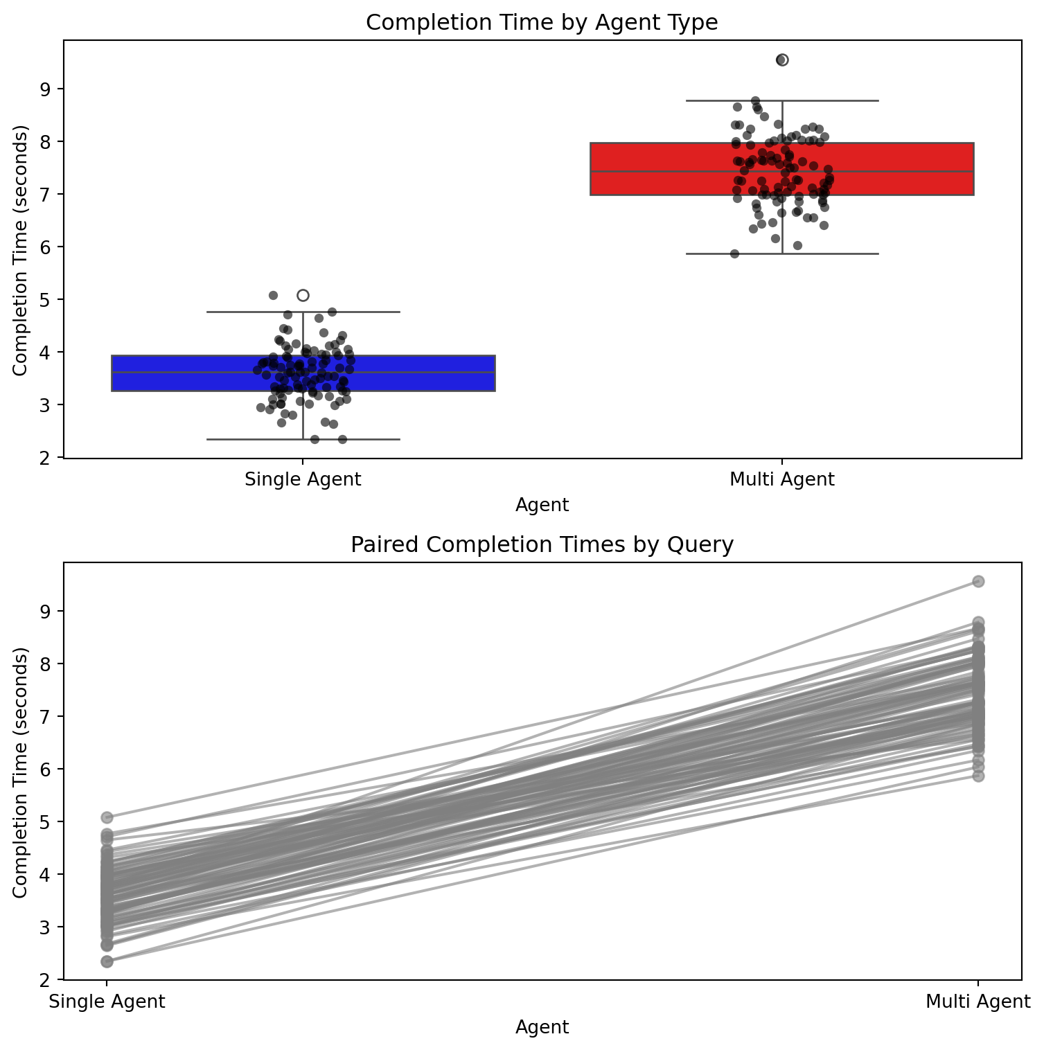
## Hypothesis Test #1 - Completion Time:
::: {.callout-note title="Hypothesis Test"}
To compare completion time between the single-agent and multi-agent systems, a **paired t-test** was used because both systems were evaluated on the same set of queries.
The paired difference for each query was defined as:
$$
d = \text{multi\_time} - \text{single\_time}
$$
A positive value of $$d$$ means the multi-agent system took longer to complete the query, which implies the single-agent system was faster.
### Null Hypothesis
$$
H_0: \mu_d = 0
$$
### Alternative Hypothesis
$$
H_A: \mu_d > 0
$$
If the p-value is less than 0.05, the null hypothesis will be rejected, providing evidence that the single-agent system is faster on average.
:::
::: {.callout-tip title="Test Statistic (Paired t‑Test)"}
The paired t‑test evaluates whether the **mean difference** in response time is significantly greater than zero.
:::
```{python}
import warnings
warnings.filterwarnings("ignore", category=UserWarning)

import pandas as pd
import numpy as np
import matplotlib.pyplot as plt
import seaborn as sns
from scipy import stats

# ---------------------------------------------------------
# Load raw data
# ---------------------------------------------------------
single = pd.read_csv("single_agent_raw.csv")
multi  = pd.read_csv("multi_agent_raw.csv")

# ---------------------------------------------------------
# Ensure required columns exist
# ---------------------------------------------------------
required_cols = ["query", "total_time"]

for col in required_cols:
    if col not in single.columns:
        raise KeyError(f"single_agent_raw.csv is missing column: {col}")
    if col not in multi.columns:
        raise KeyError(f"multi_agent_raw.csv is missing column: {col}")

# ---------------------------------------------------------
# Create query_index from row order
# ---------------------------------------------------------
single = single.reset_index(drop=True).copy()
multi = multi.reset_index(drop=True).copy()

single["query_index"] = np.arange(1, len(single) + 1)
multi["query_index"] = np.arange(1, len(multi) + 1)

# ---------------------------------------------------------
# Force total_time to numeric
# ---------------------------------------------------------
single["total_time"] = pd.to_numeric(single["total_time"], errors="coerce")
multi["total_time"]  = pd.to_numeric(multi["total_time"], errors="coerce")

# ---------------------------------------------------------
# Verify alignment by query text
# ---------------------------------------------------------
if len(single) != len(multi):
    raise ValueError(
        f"Row count mismatch: single={len(single)}, multi={len(multi)}"
    )

mismatch_rows = single["query"] != multi["query"]
if mismatch_rows.any():
    bad_idx = mismatch_rows[mismatch_rows].index[0]
    raise ValueError(
        f"Query mismatch at row {bad_idx}:\n"
        f"single = {single.loc[bad_idx, 'query']}\n"
        f"multi  = {multi.loc[bad_idx, 'query']}"
    )

# ---------------------------------------------------------
# Build paired dataframe
# ---------------------------------------------------------
paired = pd.DataFrame({
    "query_index": single["query_index"],
    "query": single["query"],
    "single_time": single["total_time"],
    "multi_time": multi["total_time"],
})

paired = paired.dropna(subset=["single_time", "multi_time"]).copy()

if len(paired) < 2:
    raise ValueError("Not enough paired observations to run a paired t-test.")

# ---------------------------------------------------------
# Descriptive statistics
# ---------------------------------------------------------
paired["diff"] = paired["multi_time"] - paired["single_time"]

desc_single = {
    "n": len(paired["single_time"]),
    "mean": paired["single_time"].mean(),
    "sd": paired["single_time"].std(ddof=1)
}

desc_multi = {
    "n": len(paired["multi_time"]),
    "mean": paired["multi_time"].mean(),
    "sd": paired["multi_time"].std(ddof=1)
}

desc_diff = {
    "n": len(paired["diff"]),
    "mean": paired["diff"].mean(),
    "sd": paired["diff"].std(ddof=1)
}

print("Descriptives")
print("Single agent:", desc_single)
print("Multi agent :", desc_multi)
print("Paired diff (multi - single):", desc_diff)

summary_df = pd.DataFrame({
    "group": ["single", "multi", "diff (multi - single)"],
    "n": [desc_single["n"], desc_multi["n"], desc_diff["n"]],
    "mean": [desc_single["mean"], desc_multi["mean"], desc_diff["mean"]],
    "sd": [desc_single["sd"], desc_multi["sd"], desc_diff["sd"]],
})
print("\nSummary table")
print(summary_df)


# ---------------------------------------------------------
# Paired t-test
# H0: mean(diff) = 0
# HA: mean(diff) > 0
# ---------------------------------------------------------
t_stat, p_two_sided = stats.ttest_rel(paired["multi_time"], paired["single_time"])

if t_stat > 0:
    p_one_sided = p_two_sided / 2
else:
    p_one_sided = 1 - (p_two_sided / 2)

# ---------------------------------------------------------
# 95% confidence interval for mean paired difference
# ---------------------------------------------------------
n = len(paired)
mean_diff = paired["diff"].mean()
sd_diff = paired["diff"].std(ddof=1)
se_diff = sd_diff / np.sqrt(n)
t_crit = stats.t.ppf(0.975, df=n - 1)

ci_low = mean_diff - t_crit * se_diff
ci_high = mean_diff + t_crit * se_diff

# ---------------------------------------------------------
# Paired effect size: Cohen's d_z
# ---------------------------------------------------------
cohens_dz = mean_diff / sd_diff if sd_diff != 0 else np.nan

print("\nPaired t-test results")
print(f"t({n-1}) = {t_stat:.4f}")
print(f"Two-sided p-value = {p_two_sided:.5f}")
print(f"One-sided p-value = {p_one_sided:.5f}")
print(f"Mean difference (multi - single) = {mean_diff:.4f}")
print(f"95% CI for mean difference = [{ci_low:.4f}, {ci_high:.4f}]")
print(f"Cohen's d_z = {cohens_dz:.4f}")

# ---------------------------------------------------------
# Interpretation
# ---------------------------------------------------------
alpha = 0.05
print("\nInterpretation")
if p_one_sided < alpha:
    print("Reject H0: there is evidence that the single-agent system is faster on average.")
else:
    print("Fail to reject H0: there is not enough evidence that the single-agent system is faster on average.")

# ---------------------------------------------------------
# Plotting dataframe
# ---------------------------------------------------------
plot_df = pd.DataFrame({
    "agent": ["Single Agent"] * len(paired) + ["Multi Agent"] * len(paired),
    "total_time": pd.concat([paired["single_time"], paired["multi_time"]], ignore_index=True),
})

# ---------------------------------------------------------
# Plots
# ---------------------------------------------------------
fig, axes = plt.subplots(2, 1, figsize=(8, 8))

# Boxplot
sns.boxplot(data=plot_df, x="agent", y="total_time", ax=axes[0], palette=["blue", "red"])
sns.stripplot(data=plot_df, x="agent", y="total_time", ax=axes[0], color="black", alpha=0.6)
axes[0].set_title("Completion Time by Agent Type")
axes[0].set_xlabel("Agent")
axes[0].set_ylabel("Completion Time (seconds)")

# Paired line plot
for _, row in paired.iterrows():
    axes[1].plot(
        ["Single Agent", "Multi Agent"],
        [row["single_time"], row["multi_time"]],
        marker="o",
        color="gray",
        alpha=0.6
    )

axes[1].set_title("Paired Completion Times by Query")
axes[1].set_xlabel("Agent")
axes[1].set_ylabel("Completion Time (seconds)")

plt.tight_layout()
plt.show()
```
## Hypothesis Test #2 - Accuracy using McNemar and Permutation tests:
We test whether the <code>single‑agent</code> and <code>multi‑agent</code> systems differ in accuracy.
Because both systems answer the **same queries**, this is a <code>paired classification comparison</code>, and McNemar’s test is appropriate.
::: {.callout-note title="Hypotheses"}
**Null Hypothesis**
$$
H_0:\ \text{Accuracy}_{\text{single}} = \text{Accuracy}_{\text{multi}}
$$
**Alternative Hypothesis**
$$
H_A:\ \text{Accuracy}_{\text{single}} \ne \text{Accuracy}_{\text{multi}}
$$
:::
::: {.callout-tip title="Test Statistic (McNemar’s Test)"}
McNemar’s test evaluates disagreement pairs:
- cases where the single‑agent is correct and the multi‑agent is wrong
- cases where the multi‑agent is correct and the single‑agent is wrong
If these counts differ significantly, accuracy differs.
:::
```{python}
import pandas as pd
import numpy as np
from statsmodels.stats.contingency_tables import mcnemar

df = pd.read_csv("correctness_scores.csv")

# Convert True/False to 1/0 if needed
df["single_correct"] = df["single_correct"].astype(int)
df["multi_correct"] = df["multi_correct"].astype(int)

# disagreement counts
b = np.sum((df["single_correct"] == 0) & (df["multi_correct"] == 1))
c = np.sum((df["single_correct"] == 1) & (df["multi_correct"] == 0))

table = [[0, b],
         [c, 0]]

result = mcnemar(table, exact=True)

print("b (single wrong, multi right):", b)
print("c (single right, multi wrong):", c)
print("statistic:", result.statistic)
print("p-value:", result.pvalue)

if result.pvalue >= 0.05:
    print("McNemar Interpretation: No statistically significant difference in accuracy.")
else:
    print("McNemar Interpretation: Statistically significant difference in accuracy.")
```
### Hypothesis #2 - Permutation Test for Accuracy:
```{python}
# Convert True/False to 1/0
df["single_correct"] = df["single_correct"].astype(int)
df["multi_correct"] = df["multi_correct"].astype(int)

# Observed difference in accuracy
obs_diff = df["single_correct"].mean() - df["multi_correct"].mean()

# Permutation test
n_permutations = 10000
perm_diffs = []

for _ in range(n_permutations):
    swapped = df.copy()

    # randomly choose which rows to swap
    mask = np.random.rand(len(df)) < 0.5

    # swap single/multi correctness for those rows
    swapped_single = swapped["single_correct"].copy()
    swapped_multi = swapped["multi_correct"].copy()

    swapped.loc[mask, "single_correct"] = swapped_multi[mask]
    swapped.loc[mask, "multi_correct"] = swapped_single[mask]

    perm_diff = swapped["single_correct"].mean() - swapped["multi_correct"].mean()
    perm_diffs.append(perm_diff)

# two-sided p-value
p_value = np.mean(np.abs(perm_diffs) >= np.abs(obs_diff))

print("Observed accuracy difference:", obs_diff)
print("Permutation p-value:", p_value)

if p_value >= 0.05:
    print("Permutation Interpretation: No evidence of an accuracy difference.")
else:
    print("Permutation Interpretation: Evidence of an accuracy difference.")
```
### Hypothesis #2 - Accuracy Summary Table:
```{python}
import pandas as pd
import numpy as np
from statsmodels.stats.contingency_tables import mcnemar

# --- Load correctness CSV ---
acc = pd.read_csv("correctness_scores.csv")

# Ensure boolean → int
acc["single_correct"] = acc["single_correct"].astype(int)
acc["multi_correct"] = acc["multi_correct"].astype(int)

# --- Basic accuracy stats ---
total_queries = len(acc)
single_correct = acc["single_correct"].sum()
multi_correct = acc["multi_correct"].sum()

single_acc = single_correct / total_queries
multi_acc = multi_correct / total_queries

# --- McNemar disagreement counts ---
b = np.sum((acc["single_correct"] == 0) & (acc["multi_correct"] == 1))
c = np.sum((acc["single_correct"] == 1) & (acc["multi_correct"] == 0))

table = [[0, b],
         [c, 0]]

mcnemar_result = mcnemar(table, exact=True)

# --- Permutation test for paired accuracy ---
obs_diff = single_acc - multi_acc
n_perm = 10000
perm_diffs = []

for _ in range(n_perm):
    swapped = acc.copy()
    mask = np.random.rand(total_queries) < 0.5

    s = swapped["single_correct"].copy()
    m = swapped["multi_correct"].copy()

    swapped.loc[mask, "single_correct"] = m[mask]
    swapped.loc[mask, "multi_correct"] = s[mask]

    perm_diffs.append(
        swapped["single_correct"].mean() - swapped["multi_correct"].mean()
    )

perm_p = np.mean(np.abs(perm_diffs) >= np.abs(obs_diff))
```
```{python}
correctness_df = pd.read_csv("correctness_scores.csv")

# Convert correctness + refusal into a single binary score
correctness_df["single_bin"] = (correctness_df["single_correct"] == 1).astype(int)
correctness_df["multi_bin"]  = (correctness_df["multi_correct"] == 1).astype(int)

b = ((correctness_df["single_bin"] == 0) & (correctness_df["multi_bin"] == 1)).sum()
c = ((correctness_df["single_bin"] == 1) & (correctness_df["multi_bin"] == 0)).sum()

table = [[0, b],
         [c, 0]]

result = mcnemar(table, exact=True)
```
```{python}
refusal_stats = pd.DataFrame({
    "Agent": ["Single Agent", "Multi Agent"],
    "Errors": [
        correctness_df["single_refusal"].sum(),
        correctness_df["multi_refusal"].sum()
    ],
    "Error Rate (%)": [
        100 * correctness_df["single_refusal"].mean(),
        100 * correctness_df["multi_refusal"].mean()
    ]
})

refusal_stats
```
```{python}
# --- Build summary table ---
summary = pd.DataFrame({
    "Metric": [
        "Total Queries",
        "Correct Answers",
        "Incorrect Answers",
        "Accuracy (%)",
        "Disagreements (b + c)",
        "McNemar b (S wrong, M right)",
        "McNemar c (S right, M wrong)",
        "Observed Accuracy Difference",
        "Permutation Test p-value"
    ],
    "Single Agent": [
        total_queries,
        single_correct,
        total_queries - single_correct,
        f"{single_acc*100:.1f}%",
        b + c,
        b,
        "",
        f"{obs_diff:.3f}",
        ""
    ],
    "Multi Agent": [
        total_queries,
        multi_correct,
        total_queries - multi_correct,
        f"{multi_acc*100:.1f}%",
        b + c,
        "",
        c,
        "",
        f"{perm_p:.3f}"
    ]
})

summary
```
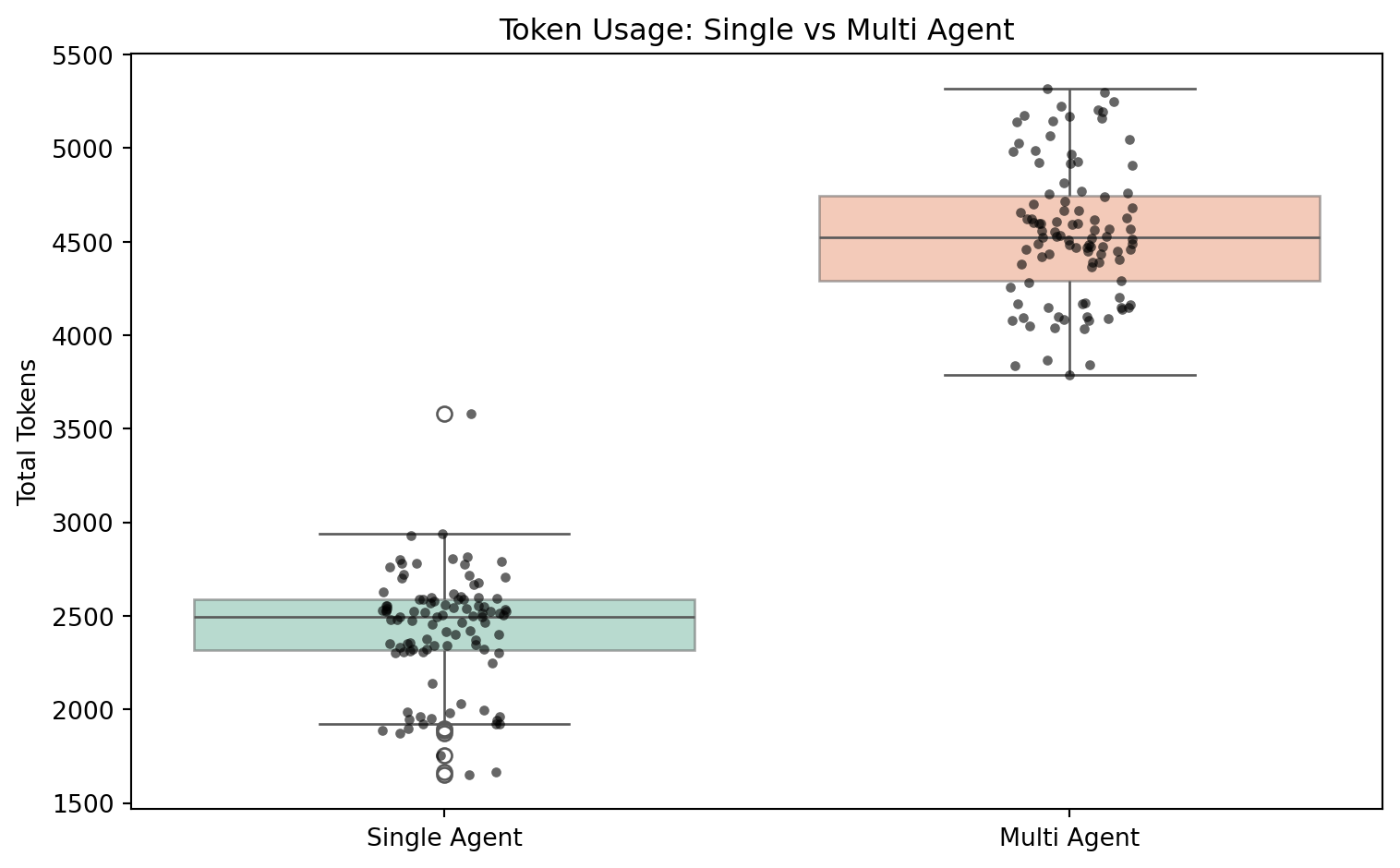
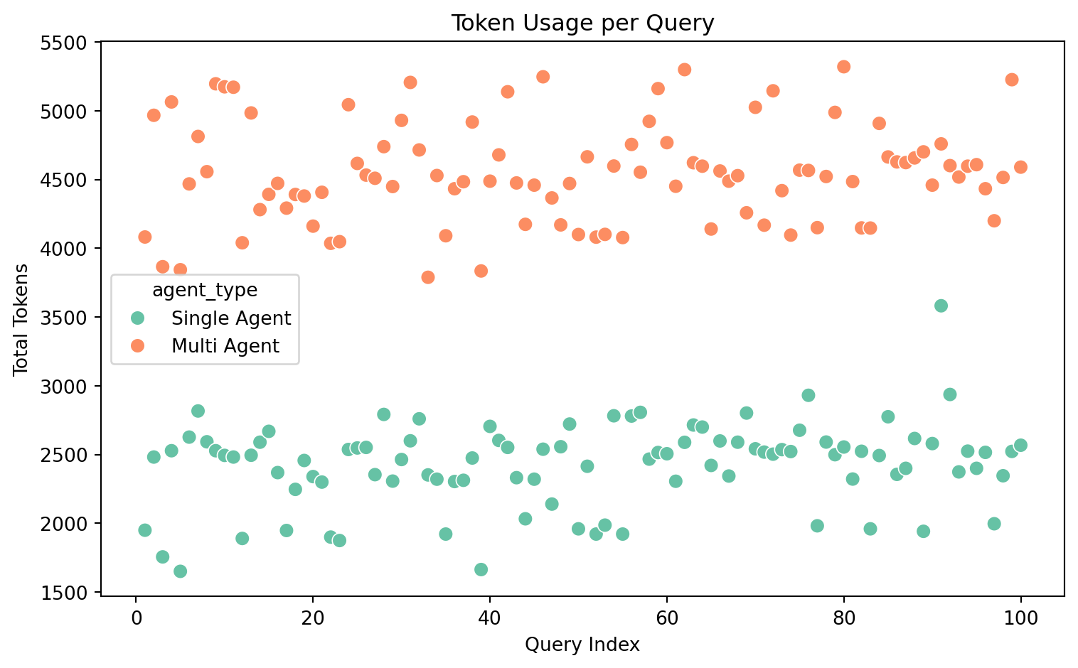
## Hypothesis Test #3 - Token Usage:
We test whether the <code>multi‑agent</code> system uses more tokens than the <code>single‑agent</code> system.
Because token counts are paired per query, a paired t‑test is appropriate.
::: {.callout-note title="Hypotheses"}
**Null Hypothesis**
$$
H_0:\ \mu_d = 0
$$
**Alternative Hypothesis**
$$
H_A:\ \mu_d > 0
$$
where
$$
d = \text{multi\_tokens} - \text{single\_tokens}
$$
:::
::: {.callout-tip title="Test Statistic (Paired t‑Test)"}
The paired t‑test evaluates whether the **mean difference** in token usage is significantly greater than zero.
:::
```{python}
import pandas as pd
import matplotlib.pyplot as plt
import seaborn as sns

# Load CSVs
single = pd.read_csv("single_agent_raw.csv")
multi = pd.read_csv("multi_agent_raw.csv")

# Add agent labels
single["agent_type"] = "Single Agent"
multi["agent_type"] = "Multi Agent"

# --- Ensure query_index exists ---
single["query_index"] = range(1, len(single) + 1)
multi["query_index"] = range(1, len(multi) + 1)

# Combine
df = pd.concat([single, multi], ignore_index=True)

# Extract token columns
single_tokens = single["tokens_total"]
multi_tokens = multi["tokens_total"]

# Paired differences
diff = multi_tokens - single_tokens
```
```{python}
# Summary statistics
desc_stats = pd.DataFrame({
    "Metric": [
        "Mean Tokens",
        "Median Tokens",
        "Std Dev",
        "Min",
        "Max",
        "IQR",
    ],
    "Single Agent": [
        single_tokens.mean(),
        single_tokens.median(),
        single_tokens.std(),
        single_tokens.min(),
        single_tokens.max(),
        single_tokens.quantile(0.75) - single_tokens.quantile(0.25),
    ],
    "Multi Agent": [
        multi_tokens.mean(),
        multi_tokens.median(),
        multi_tokens.std(),
        multi_tokens.min(),
        multi_tokens.max(),
        multi_tokens.quantile(0.75) - multi_tokens.quantile(0.25),
    ]
})

# Difference summary
diff_stats = pd.DataFrame({
    "Statistic": ["Mean Difference (multi - single)", "Median Difference"],
    "Value": [diff.mean(), diff.median()]
})

desc_stats, diff_stats
```
```{python}
# --- Boxplot ---
plt.figure(figsize=(8, 5))

sns.boxplot(
    data=df,
    x="agent_type",
    y="tokens_total",
    palette="Set2",
    showcaps=True,
    boxprops={'alpha':0.5}
)

sns.stripplot(
    data=df,
    x="agent_type",
    y="tokens_total",
    color="black",
    size=4,
    jitter=True,
    alpha=0.6
)

plt.title("Token Usage: Single vs Multi Agent")
plt.ylabel("Total Tokens")
plt.xlabel("")
plt.tight_layout()
plt.show()
```
```{python}
# --- Scatter plot ---
plt.figure(figsize=(8, 5))
sns.scatterplot(
    data=df,
    x="query_index",
    y="tokens_total",
    hue="agent_type",
    palette="Set2",
    s=60
)
plt.title("Token Usage per Query")
plt.ylabel("Total Tokens")
plt.xlabel("Query Index")
plt.tight_layout()
plt.show()
```
### Token Usage Summary
```{python}
# Load your result files
## Token Usage Summary

# Load CSVs
single = pd.read_csv("single_agent_raw.csv")
multi = pd.read_csv("multi_agent_raw.csv")
baseline = pd.read_csv("baseline_raw.csv")

# Compute totals
single_total = single["tokens_total"].sum()
multi_total = multi["tokens_total"].sum()
baseline_total = baseline["tokens_total"].sum()

# Grand total
total_tokens = single_total + multi_total + baseline_total

# Pricing (adjust to your model)
price_per_million = 2.5
cost = (total_tokens / 1_000_000) * price_per_million

# Pretty output
print(" Token Usage by Agent")
print(f"- Single-Agent: {single_total:,} tokens")
print(f"- Multi-Agent:  {multi_total:,} tokens")
print(f"- Baseline:     {baseline_total:,} tokens")
print()
print(" Total Token Usage")
print(f"- Total tokens: {total_tokens:,}")
print(f"- Estimated cost: ${cost:.4f}")
```
# Interactive Plots
```{python}
import importlib
import plots
importlib.reload(plots)

from plots import (
    interactive_query_health,
    interactive_completion_time,
    interactive_tool_usage,
    interactive_answer_length,
    interactive_answer_comparison,
    interactive_token_usage
)
```
```{python}
tmp = (
    interactive_completion_time(single_df, multi_df),
    interactive_tool_usage(single_raw, multi_raw),
    interactive_answer_length(single_raw, multi_raw),
    interactive_query_health(single_raw),
    interactive_query_health(multi_raw),
    interactive_token_usage(single_raw, multi_raw)
)
```
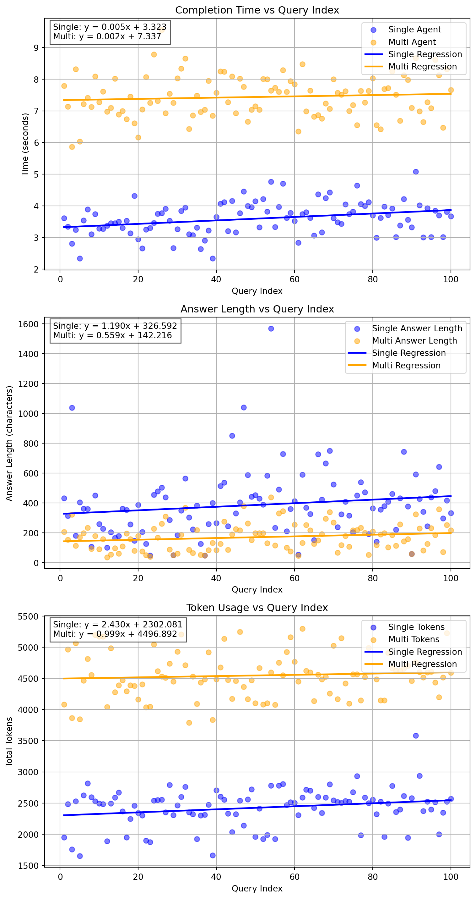
## Completion Time
```{python}
#| echo: false
#| format: html
fig_completion = interactive_completion_time(single_df, multi_df)
fig_completion
```
## Answer Length:
```{python}
#| echo: false
#| format: html
fig_answer = interactive_answer_length(single_raw, multi_raw)
fig_answer
```
## Token Usage:
```{python}
#| echo: false
#| format: html
fig_answer = interactive_token_usage(single_raw, multi_raw)
fig_answer
```
## Dashboard Summary
```{python}
from plots import plot_dashboard

fig = plot_dashboard(single_raw, multi_raw)
```
# Real Life Uses:
## Sports:
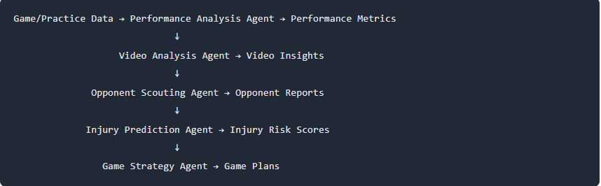
@reputagent_sports_analytics
## Medicine:
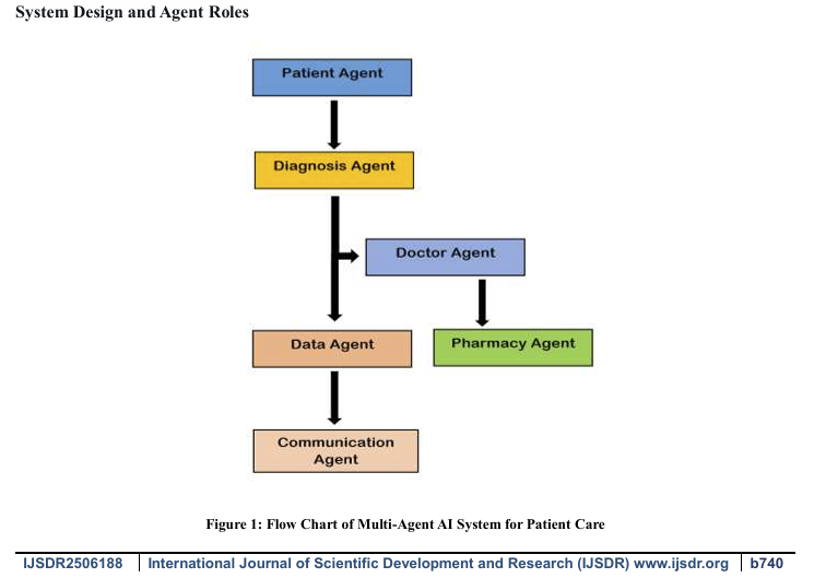
@Saeed2025MASHealthcare
# Key takeaways:
- API integration ability
- Agents are efficient on their own or part of a multi agent system.
- Cost goes up quite a bit when using a multi agent system.
- Extremely low percentage of incorrect answers/hallucinations.
- Can be applied to anywhere.
# Conclusion:
Overall, the single agent and multi agent outperform your standard LLM. When it comes down to whether a single or multi agent is better, you could really go either way.
Based on my data, a single agent would be much faster per query but the multi would be more accurate. As always, cost is a big factor in deciding which to use. Both have the major appeals of an LLM-Agent.
# Further Reading
- LLM-Agent Capabilities - https://www.geeksforgeeks.org/artificial-intelligence/llm-agents/
# DISCLAIMER:
***Never blindly trust AI! Keep those critical thinking skills on hand!***
# Questions?
# References